Population genetics analyses
Developed by: Julian Catchen, Nicolas Rochette
Adapted by: Ludovic Dutoit
Goals
Learn to run basic population genetics analyses
Structure
Our goal now is to export a subset of loci for analysis in Structure, which analyzes the distribution of multi-locus genotypes within and among populations in a Bayesian framework to make predictions about the most probable population of origin for each individual. The assignment of each individual to a population is quantified in terms of Bayesian posterior probabilities, and visualized via a plot of posterior probabilities for each individual and population.
A key user defined parameter is the hypothesized number of populations of origin which is represented by K. Sometimes the value of K is clear from from the biology, but more often a range of potential K-values must be explored and evaluated using a variety of likelihood based approaches to decide upon the ultimate K. In the interests of time we won’t be exploring different values of K here, but this will be a key step for your own datasets. In addition, Structure takes a long time to run on the number of loci generated in a typical RAD data set because of the MCMC algorithms involved in the Bayesian computation. We therefore want to choose a random subset of loci that are well represented across our three populations. Despite ‘downsampling’, this random subset contains more than enough information to define population structure.
The final stage of the Stacks pipeline is to run the populations program. Now, we want to execute just populations, rather than the full Stacks pipeline, to specify filters that will give us only the most well-represented loci. populations is a very useful piece of software both for filtering and for outputting population genetics files and parameter estimates. It can work with non-stacks generated data too.
The help for populations is here
• Since we won’t be able to use all loci for our quick downstream analysis today, we will run populations again, specifying that loci must be present in at least 80% of individuals in all three populations to cut down on the total number of loci in the directory).
• Make sure to output a structure file and a .vcf file as well. We might be coming back to that .vcf file later today.
• Specify output_refmap as the path to the directory containing the Stacks files
• Also specify output_refmap as the output folder
This command is now ready, and assuming you are in the GBS folder, run it! It is a quickie, so no need to put it in a batch job.
How many SNPs do you have left? We want to select 1,000 loci randomly from the results to run a relatively quick Structure analysis. We will save these loci into a file. We can easily do this using the shell given a list of catalog IDs output in the previous step. The populations.sumstats.tsv file gives a list of all polymorphic loci.
With the help of the instructions below, use the cat, grep, cut, sort, uniq, shuf, and head commands to generate a list of 1,000 random loci. Save this list of loci as whitelist.txt, so that we can feed it back into populations. This operation can be done in a single shell command. That sounds challenging, but the instructions below should help you create one command with several pipes to create that whitelist.txt file. The idea of a pipe is to connect commands using | e.g. command 1 | command 2 outputs the content of command 1 into command 2 instead of outputting it to the screen.
Let’s create that command step by step:
• First, use cat to concatenante output_refmap/populations.sumstats.tsv (stream it to the next command)
• Then, add a | in your command and use the command grep with -v to exclude all headers (i.e. -v stands for exclude, we want to exclude all the lines with “#”)
• Add another | and select the first column with cut -f 1
• Then using two more pipes, use sort before using uniq. uniq will collapse succesive identical lines into single lines, so that you have one line per locus. Lucky us, those two commands don’t require any arguments.
• Now try adding shuf which will mix all these lines all over.
• Select the first one thousand lines with head -n 1000 and put it all into whitelist.txt. (hint: use “>” to redirect into a file). Do not worry about the shuf: write error: Broken pipe, it is simply because head stops the command before the end.
You got this! If you are new to bash, I am sure writing this command seemed impossible on Monday, so take a minute to congratulate yourself on the progress made even if you required a little help!
Now we will execute populations again, this time feeding back in the whitelist you just generated. Check out the help of populations to see how to use a white list. This will cause populations to only process the loci in the whitelist.txt.
• Specify that a structure output file be included this time.
• Specify --write-single-snp so that only one snp per locus is output as we need genetically unlinked SNPs (i.e. statistically)
• Finally, you will need to again specify the population map so that this information is passed into the structure output file. This time we will specify the population map with the proper population information. That file is at /nesi/project/nesi02659/obss_2020/resources/day3/complete_popmap.txt. You can copy this file here, link it, or simply specify the full path, your call! All of these 3 solutions should work.
• We’ve run commands to generate the structure file two times now, but how many structure files are there in the stacks directory? If you wanted to save several different vcf and structure files generated using different populations options, what would you have to do?
Create a new directory called structure within the GBS folder and copy the structure output file that Stacks generated to this directory. cd into your new structure directory.
• Edit the structure output file to remove the comment line (i.e. first line in the file, starts with “#”).
• The parameters to run structure (with value of K=3) have already been prepared, you can find them here: /nesi/project/nesi02659/obss_2020/resources/day3/mainparams and /nesi/project/nesi02659/obss_2020/resources/day3/extraparams. Copy them into your structure directory as well.
• So far, when we’ve gone to run programs, we’ve been able to use module spider to figure out the program name, and then module load program_name to get access to the program and run it. Do it one more time for structure
• run structure by simply typing structure
Do you see WARNING! Probable error in the input file.? In our mainparams file it says that we have 1000 loci, but due to filters, it is possible that the populations module of Stacks actually output less than the 1000 loci we requested in whitelist.txt. In the output of populations.log in your output_refmap directory, how many variant sites remained after filtering? This is the number of loci actually contained in your structure file. You will need to adjust the number of loci in the mainparams file to match this exact Stacks output.
Structure Visualisation
• Once you ran structure successfully. It is time to visualise the results. We will do that in R.
• Open an R launcher, be careful to open R 4.0.1 to have access to all the needed packages.
setwd("/nesi/project/nesi02659/obss_2020/users/<username>/GBS/structure") # Get R to your own structure folder
library("pophelper")# load plotting module for structure http://www.royfrancis.com/pophelper/reference/readQ.html
data<-readQ("populations.structure.out_f",filetype = "structure",indlabfromfile=TRUE)
plotQ(data,showindlab = TRUE,useindlab=TRUE)  # http://www.royfrancis.com/pophelper/reference/readQ.html
• That should create a structure image in your structure folder. Use the path navigator on the left to reach your folder to be able to visualise the picture by double-clicking on it.
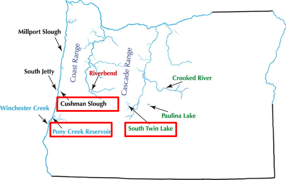
• Are the three Oregon threespine stickleback populations related to one another? How can you tell? Use the population labels on the map below to think about it (cs: Cushman Slough , pcr: Poney Creek reservoir, stl: South Twin Lake; original paper)
Congrats, you just finished our tutorial for the assembly of RAD-Seq data. Here are a few things you could do to solidify your learning from today.
Extra activities
• You could play a bit with the parameters of plotQ() at http://www.royfrancis.com/pophelper/reference/readQ.html to make a prettier figure.
• You could spend a bit of time going through and making sure you understand the set of steps we did in those few exercises.
• You could try running this set of analyses on a de novo dataset. You can use the one you generated yourself or the -M 2 dataset that is in /nesi/project/nesi02659/obss_2020/resources/day3/output_denovo_M2.
• You could have a look at this tutorial. It is a small tutorial I wrote previously that goes over a different set of population genetics analyses in R. You could even try reproducing it using the vcf you generated above. The vcf for the set of analyses presented in that code can be downloaded here should you want to download it.