Exploration of population structure using GBS
Ludovic Dutoit 2/7/2019
Summary
In this quick example script, we will examplify basic population genetics analyses of a GBS a dataset of Gobiomorphus cotidianus between two New Zealand lake: Wakatipu (WP) and Wanaka (WK).
For any questions or access to data files to dutoit.ludovic@gmail.com. The pipeline require several R packages for different parts that should be installed in your system. The links below refer to all the installations:
Loading files
require("pcadapt")
## Warning: package 'pcadapt' was built under R version 3.5.2
data <- read.pcadapt("populations.snps.vcf", type = "vcf") # New dataset https://github.com/ldutoit/bully_gbs/blob/master/populationstructure_tuto/populations.snps.vcf
## No variant got discarded.
## Summary:
##
##  - input file:               populations.snps.vcf
##  - output file:              /var/folders/1g/hdrjtwrj77b1g8ll485bl2sw0000gq/T//RtmpXyQUBh/file1212c64cfe02d.pcadapt
##
##  - number of individuals detected:   94
##  - number of loci detected:      9605
##
## 9605 lines detected.
## 94 columns detected.
94 individuals and 9605 variants.
Now, onto loading some metadata:
##Load some metadata
metadata<-read.table("metadata_clean.txt",h=T)# # (This fileis available https://github.com/ldutoit/)bully_gbs/blob/master/populationstructure_tuto/metadata/metadata_clean.txt)
head(metadata)
##    sample   lake depth   group sex
## 1 WK16-02 Wanaka    90    Deep   m
## 2 WK16-16 Wanaka    90    Deep   m
## 3 WK16-33 Wanaka    60    Deep   f
## 4 WK16-66 Wanaka    15 Shallow   f
## 5 WK16-80 Wanaka     5 Shallow   f
## 6 WK16-97 Wanaka     5 Shallow   m
Basic statistics
Let’s get some basic population stats (Fst, Ho)
require("hierfstat") ## install those packages first https://github.com/jgx65/hierfstat
## Loading required package: hierfstat
require("vcfR")
## Loading required package: vcfR

##
##    *****       ***   vcfR   ***       *****
##    This is vcfR 1.8.0
##      browseVignettes('vcfR') # Documentation
##      citation('vcfR') # Citation
##    *****       *****      *****       *****
require("poppr")
## Loading required package: poppr

## Warning: package 'poppr' was built under R version 3.5.2

## Loading required package: adegenet

## Loading required package: ade4

##
##    /// adegenet 2.1.1 is loaded ////////////
##
##    > overview: '?adegenet'
##    > tutorials/doc/questions: 'adegenetWeb()'
##    > bug reports/feature requests: adegenetIssues()

##
## Attaching package: 'adegenet'

## The following object is masked from 'package:hierfstat':
##
##     read.fstat

## This is poppr version 2.8.3. To get started, type package?poppr
## OMP parallel support: available
# a bit of play around wqith convewrsion to get a vcf into hierfstat
dataVCF<- read.vcfR("populations.snps.vcf", verbose = T)
## Scanning file to determine attributes.
## File attributes:
##   meta lines: 14
##   header_line: 15
##   variant count: 9605
##   column count: 103
##
Meta line 14 read in.
## All meta lines processed.
## gt matrix initialized.
## Character matrix gt created.
##   Character matrix gt rows: 9605
##   Character matrix gt cols: 103
##   skip: 0
##   nrows: 9605
##   row_num: 0
##
Processed variant 1000
Processed variant 2000
Processed variant 3000
Processed variant 4000
Processed variant 5000
Processed variant 6000
Processed variant 7000
Processed variant 8000
Processed variant 9000
Processed variant: 9605
## All variants processed
geninddata<-vcfR2genind(dataVCF)# convert data from vcf object to genind
geninddata@pop<-(metadata[,2]) # assign populations
head(geninddata@pop)
## [1] Wanaka Wanaka Wanaka Wanaka Wanaka Wanaka
## Levels: Wakatipu Wanaka
#Make 4 pops, shallow and deep for both lakes
hierfstatdataall <-genind2hierfstat(geninddata,pop=paste(metadata[,2],metadata[,4],sep=""))
levels(hierfstatdataall$pop) # checking we have for pops
## [1] "WakatipuDeep" "WakatipuShallow" "WanakaDeep" "WanakaShallow"
basic.stats(hierfstatdataall)$overall # get the basic stats
##      Ho      Hs      Ht     Dst     Htp    Dstp     Fst    Fstp     Fis
##  0.1281  0.1272  0.1354  0.0082  0.1381  0.0109  0.0604  0.0790 -0.0071
##    Dest
##  0.0125
Some important information in there! Let’s also do a pwiarwise Fst Matrix based on Weir and Cockerham, 1984.
matrix_4_depth_fst<-as.matrix(genet.dist(hierfstatdataall,method="WC84"))
colnames(matrix_4_depth_fst)<-levels(hierfstatdataall$pop)
rownames(matrix_4_depth_fst)<-levels(hierfstatdataall$pop)
matrix_4_depth_fst
##                  WakatipuDeep WakatipuShallow  WanakaDeep WanakaShallow
## WakatipuDeep     0.0000000000   -0.0002000228 0.097651865   0.106026741
## WakatipuShallow -0.0002000228    0.0000000000 0.116983828   0.126122435
## WanakaDeep       0.0976518655    0.1169838285 0.000000000   0.001426047
## WanakaShallow    0.1060267412    0.1261224346 0.001426047   0.000000000
Little structure by depth, only between lakes
Population Structure
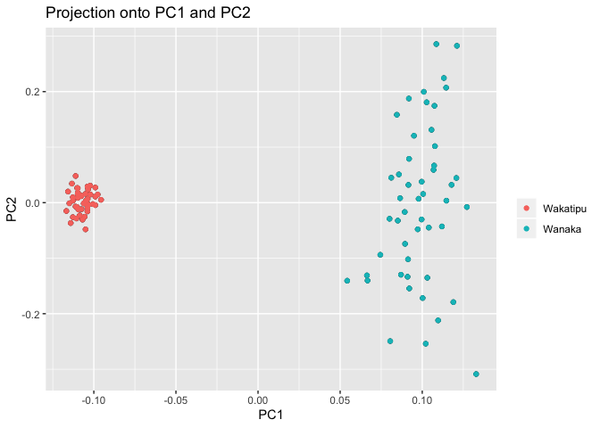
Now that we have all the data and metadat loaded in and that we have looked some basic stats, let’s have a quick look at the general population structure. We will make a PCA, colored by lake using the pcadapt package.
x <- pcadapt(input = data, K = 20)
rownames(x$scores)<-metadata[,1]
colnames(x$scores)<-paste("PC",1:20,sep="")
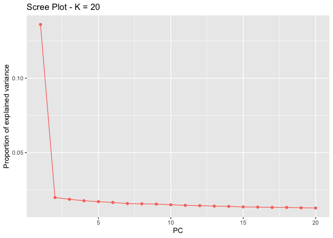
plot(x, option = "screeplot")

plot(x, option = "scores", pop=metadata$lake) # you can put any factor as the group, here we look at the two lakes.

Again, we find the lake structure.
fastStructure analysis
“fastStructure is an algorithm for inferring population structure from large SNP genotype data. It is based on a variational Bayesian framework for posterior inference and is written in Python2.x.”
File conversion The conversion from vcf to faststructure input files is done using PGDspider2.1.1.5 (http://www.cmpg.unibe.ch/software/PGDSpider/).
Note that once converted the file, faststructure arguments should not have the extension. Below populations.snps is referring to populations.snps.str.
fastStructure run The fastStructure code below is bash and should be run in the shell not in R. If you are not sure where you are located in your computer you can obtain with the following R command:
getwd()
## [1] "/Users/dutlu42p/repos/mahuika/bully_gbs/populationstructure_tuto"
We run it for K=2 to K=10 as there is 10 sampling locations. It makes no sense to go above 10.
#create output folders for the analysis and for later plots
mkdir faststructure_exploration plots
module load fastStructure  # speciic to the way faststructure  is installed on the NeSI infrastructure
structure.py -K 2  --input=populations.snps --output=faststructure_exploration/populations.snps --format=str
structure.py -K 3  --input=populations.snps --output=faststructure_exploration/populations.snps --format=str
structure.py -K 4  --input=populations.snps --output=faststructure_exploration/populations.snps --format=str
structure.py -K 5  --input=populations.snps --output=faststructure_exploration/populations.snps --format=str
structure.py -K 6  --input=populations.snps --output=faststructure_exploration/populations.snps --format=str
structure.py -K 7  --input=populations.snps --output=faststructure_exploration/populations.snps --format=str
structure.py -K 8  --input=populations.snps --output=faststructure_exploration/populations.snps --format=str
structure.py -K 9  --input=populations.snps --output=faststructure_exploration/populations.snps --format=str
structure.py -K 10  --input=populations.snps --output=faststructure_exploration/populations.snps --format=str

chooseK.py --input=faststructure_exploration/populations.snps
Model complexity that maximizes marginal likelihood = 2
Model components used to explain structure in data = 2
The choose K function suggests K=2 that only the structure between lake is clearly visible, let’s see how it looks like in practice:
require("pophelper") # to install: http://www.royfrancis.com/pophelper/articles/index.html
## Loading required package: pophelper

## Loading required package: ggplot2

## Warning: package 'ggplot2' was built under R version 3.5.2

## pophelper v2.2.9 ready.
ffiles <- list.files(path="faststructure_exploration/",pattern="meanQ")[grep(paste("populations.snps",sep=""),perl=T,list.files(path="faststructure_exploration/",pattern= "meanQ"))]#simply a vector of the faststructure files we want to read
ffiles
## [1] "populations.snps.10.meanQ" "populations.snps.2.meanQ"
## [3] "populations.snps.3.meanQ"  "populations.snps.4.meanQ"
## [5] "populations.snps.5.meanQ"  "populations.snps.6.meanQ"
## [7] "populations.snps.7.meanQ"  "populations.snps.8.meanQ"
## [9] "populations.snps.9.meanQ"
flist <- readQ(files=paste("faststructure_exploration/",ffiles,sep=""))
## add metadata to each file
indcodes <- metadata[,1]
      for (i in 1:length(flist)){
          rownames(flist[[i]]) <-indcodes
      }

  #Plot it into the folder
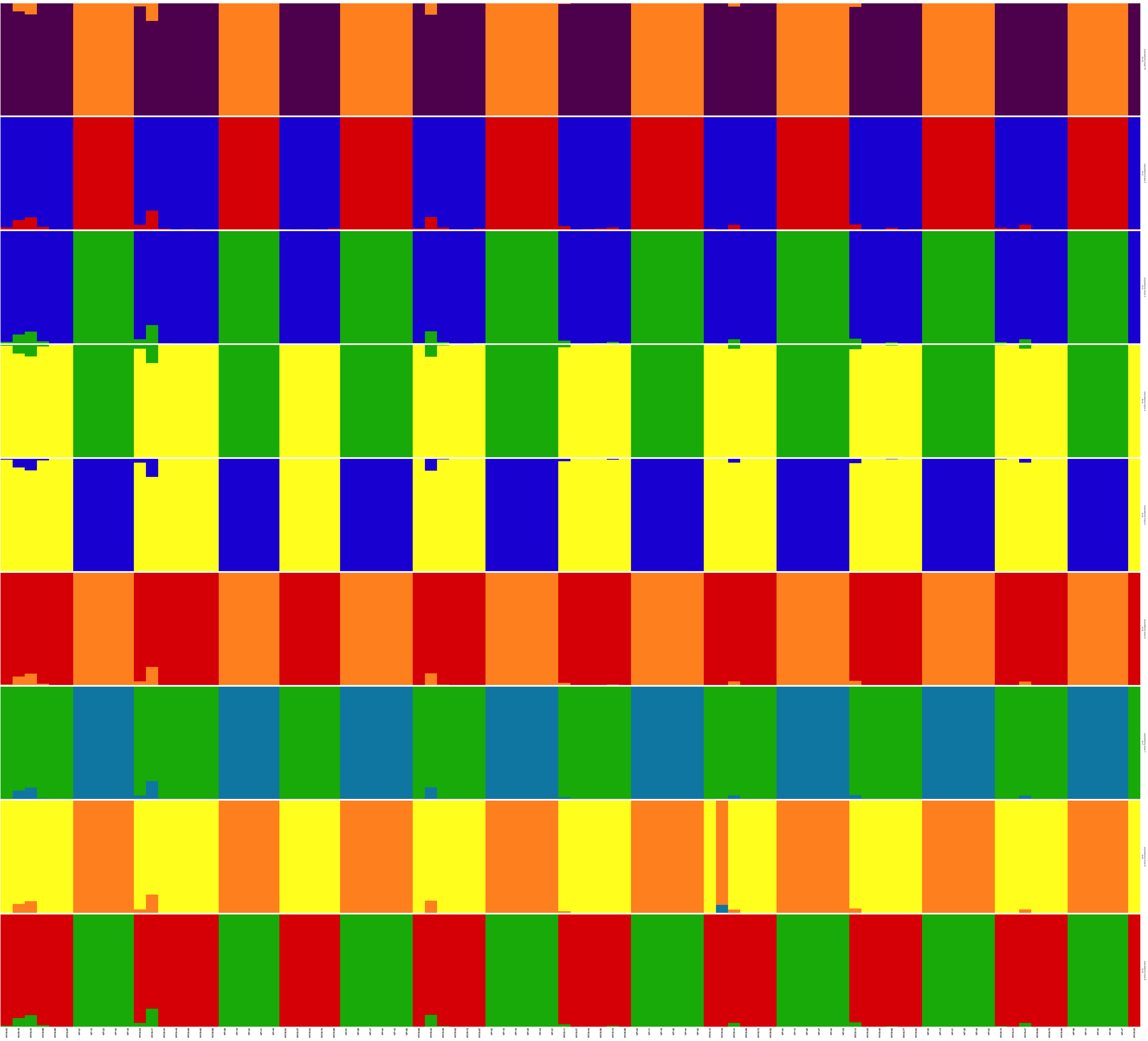
plotQ(flist,imgoutput="join",showindlab=T,useindlab=T,height=7,width=70,grplabangle=0,,ordergrp=T,exportpath= "faststructureK2toK10")
## Drawing plot ...

## faststructureK2toK10Joined9Files-20200220121348.png exported.

Looking at that file, We can clearly see the two clusters regardless of the set K. But individuals are not ordered by populations. Let’s fix that to get pretty plots. Altough I could have provided us with clean and ordered files to start with, this is a common issue so let’s go together through re-ordering faststructure files.
#determine proper order numerically from old order
indices_of_wanaka_samples<-grep("WK",metadata[,1]) #columns number we want in group 1
indices_of_wakatipu_samples<-grep("WP",metadata[,1])  #columns number we want in group 1
new_order_of_the_94_samples <- c(indices_of_wanaka_samples,indices_of_wakatipu_samples)
#find files
filestoread<-paste("faststructure_exploration/",list.files(path="faststructure_exploration/",pattern="meanQ")[grep(paste("populations.snps",sep=""),perl=T,list.files(path="faststructure_exploration/",pattern= "meanQ"))],sep="")#simply a vector of the faststructure files we want to read
print(filestoread)# The 9 files I need to reorder to check visually!
## [1] "faststructure_exploration/populations.snps.10.meanQ"
## [2] "faststructure_exploration/populations.snps.2.meanQ"
## [3] "faststructure_exploration/populations.snps.3.meanQ"
## [4] "faststructure_exploration/populations.snps.4.meanQ"
## [5] "faststructure_exploration/populations.snps.5.meanQ"
## [6] "faststructure_exploration/populations.snps.6.meanQ"
## [7] "faststructure_exploration/populations.snps.7.meanQ"
## [8] "faststructure_exploration/populations.snps.8.meanQ"
## [9] "faststructure_exploration/populations.snps.9.meanQ"
#Eeorder every single file according to proper order
for (filename in filestoread){
  tempdata<-read.table(filename,h=F) #Read old file
  tempdata<-tempdata[new_order_of_the_94_samples,] #reorder
  newfilename = paste(strsplit(filename,".populations")[[1]][1],"/","reordered",strsplit(filename,".populations")[[1]][2],sep="")
  write.table(tempdata,newfilename,quote=F,col.names=F,row.names=F,sep="\t")
    print(paste(filename,"rewriting as",newfilename),sep="")

}
## [1] "faststructure_exploration/populations.snps.10.meanQ rewriting as faststructure_exploration/reordered.snps.10.meanQ"
## [1] "faststructure_exploration/populations.snps.2.meanQ rewriting as faststructure_exploration/reordered.snps.2.meanQ"
## [1] "faststructure_exploration/populations.snps.3.meanQ rewriting as faststructure_exploration/reordered.snps.3.meanQ"
## [1] "faststructure_exploration/populations.snps.4.meanQ rewriting as faststructure_exploration/reordered.snps.4.meanQ"
## [1] "faststructure_exploration/populations.snps.5.meanQ rewriting as faststructure_exploration/reordered.snps.5.meanQ"
## [1] "faststructure_exploration/populations.snps.6.meanQ rewriting as faststructure_exploration/reordered.snps.6.meanQ"
## [1] "faststructure_exploration/populations.snps.7.meanQ rewriting as faststructure_exploration/reordered.snps.7.meanQ"
## [1] "faststructure_exploration/populations.snps.8.meanQ rewriting as faststructure_exploration/reordered.snps.8.meanQ"
## [1] "faststructure_exploration/populations.snps.9.meanQ rewriting as faststructure_exploration/reordered.snps.9.meanQ"
#We also need to reorder the metadat
indcodes_reordered<-paste(metadata[new_order_of_the_94_samples,1],metadata[new_order_of_the_94_samples,2],metadata[new_order_of_the_94_samples,3],"m",sep="_")
We recreated all these re-ordered files. Let’s make the clean plots
ffiles <- list.files(path="faststructure_exploration/",pattern="meanQ")[grep(paste("reor",sep=""),perl=T,list.files(path="faststructure_exploration/",pattern= "meanQ"))] #simply a vector of the faststructure files we want to read
flist <- readQ(files=paste("faststructure_exploration/",ffiles,sep=""))
print(ffiles)
## [1] "reordered.snps.10.meanQ" "reordered.snps.2.meanQ"
## [3] "reordered.snps.3.meanQ"  "reordered.snps.4.meanQ"
## [5] "reordered.snps.5.meanQ"  "reordered.snps.6.meanQ"
## [7] "reordered.snps.7.meanQ"  "reordered.snps.8.meanQ"
## [9] "reordered.snps.9.meanQ"
## add metadata
      for (i in 1:length(flist)){
          rownames(flist[[i]]) <-indcodes_reordered
      }
  #Plot it into the folder
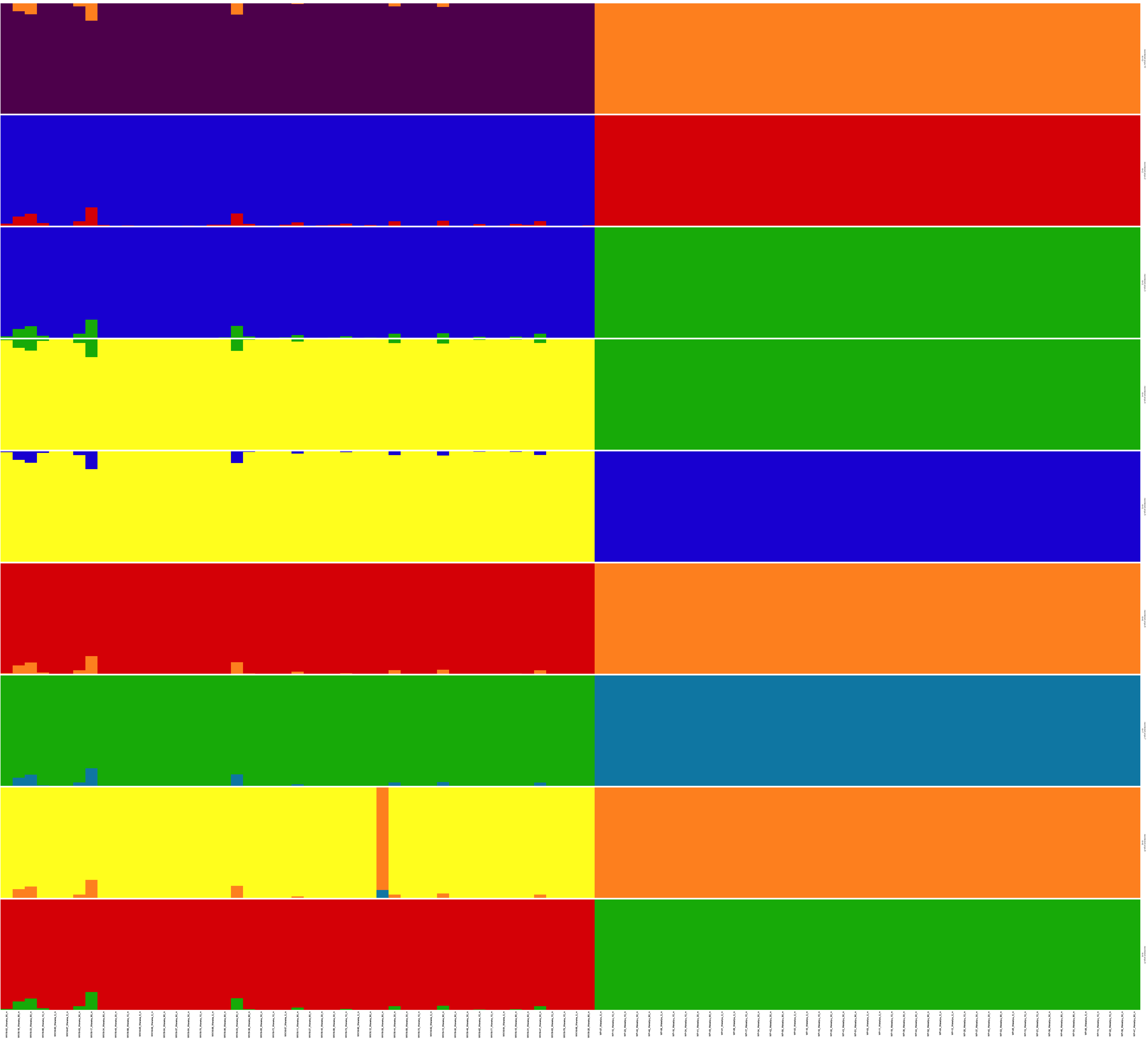
plotQ(flist,imgoutput="join",showindlab=T,useindlab=T,height=7,width=70,grplabangle=0,,ordergrp=T)
## Drawing plot ...

## Joined9Files-20200220121405.png exported.

Great! Rows are K = 2 to K = 10. and the individuals are now sorted by lake. We’ll make a final plot with only K=2 that looks a bit prettier:
plotQ(flist[2],imgoutput ="sep", showindlab=T,useindlab=T ,height=7,width=35,grplabangle=0,exportpath="K2", rainbow(2),showdiv=TRUE,clustercol=c("red","blue"),divcol="white",divtype=1,divsize=1,sortind=NA,grplab=NA)
## Drawing plot ...

## K2reordered.snps.2.png exported.

Well done!