2020-spring-school-GBS

Project maintained by ldutoit Hosted on GitHub Pages — Theme by mattgraham

Data101: From raw data to individual samples files

Developed by: Julian Catchen, Nicolas Rochette

Adapted by: Ludovic Dutoit

Goal

The goal of this first exercise is to take you from raw reads data to individual sample files.

We will check the quality of the data
Assign reads to individual samples

Working with single-end reads

The first step in the analysis of all short-read sequencing data, including RAD-seq data, is removing low quality sequences and separating out reads from different samples that were individually barcoded. This ‘de-multiplexing’ serves to associate reads with the different individuals or population samples from which they were derived.

Let’s organise our space, get comfortable moving around, and copy our data :

• Log into Jupyter at https://jupyter.nesi.org.nz/hub/login. Not sure how to do it? Just follow the instructions jupyter_hub.md

• For each exercise, you will set up a directory structure on the remote server that will hold your data and the different steps of your analysis. We will start by making the directory GBS in your working space, so let’s cd (change directory) to your working location:
```
cd /nesi/project/nesi02659/obss_2020/users/<yourusername>/
```
OR from the launch of the Jupyter terminal:
```
cd obss_2020/users/<yourusername>/
```
NOTE: If you get lost at any time today, you can always cd to your directory following the upper link.

• Once there, create the directory GBS and then change directory into GBS:
```
 mkdir GBS
 cd GBS
```
The exercise from now on is hands-on: the instructions are here to guide you through the process but you will have to come up with the specific commands yourself. Fear not, the instructions are there to help you and the room is full of friendly faces to help you get through it.
We will create more subdirectories to hold our analyses. Be careful that you are reading and writing files to the appropriate directories within your hierarchy. You’ll be making many directories, so stay organized! We will name the directories in a way that corresponds to each stage of our analysis and that allows us to remember where all our files are! A well organized workspace makes analyses easier and prevents data from being accidentally overwritten.

• First let’s make a few directories. In GBS, create a directory called dataprep to contain all the data for this exercise. Inside that directory dataprep we will create two additional directories: lane1 and samples.

• As a check that we’ve set up our workspace correctly, go back to your GBS directory (hint: cd .. goes up one level) and use the ls -R (the ls command with the recursive flag). It should show you the following (./ is a placeholder for ‘current directory’):
```
 .:
 dataprep

 ./dataprep:
 lane1  samples

 ./dataprep/lane1:

 ./dataprep/samples:
```
• Copy the dataset containing the raw reads to your lane1 directory. The dataset is the file /nesi/project/nesi02659/obss_2020/resources/day3/lane1.tar (hint: cp /path/to/what/you/want/to/copy /destination/you/want/it/to/go)

• cd to your lane1 folder to extract/unzip the content of this tar archive file. This is a compressed (aka ‘zip’) folder. We realise that we have not told you how to do extract/unzip tar files! But a quick look to a friendly search engine will show you how easy it is to find this kind of information on basic bash commands (your instructors still spend a lot of time doing this themselves! hint: you might try searching for “How to extract a tar archive”)
Have a look at what is there now (hint: ls). These gz-compressed fastq files have milions of reads in them, too many for you to examine in a spreadsheet or word processor. However, we can examine the contents of the set of files in the terminal (the less command may be of use).
Let’s have a closer look at this data. Over the last couple of days, you learnt to run FastQC to evaluate the quality of the data. Run it on these files. Load the module first and then run FastQC over all the gzipped file. We will help you out with these commands, but bonus question as you work through these: What do the commands module spider, module load, module purge do?
```
 module purge
 module spider fastqc 
 module load FastQC
 fastqc *gz
```
Explanations of this code: module purge get rids of any pre-existing potentially conflicting modules. module spider searches for modules e.g. module spider fastqc looks for a module called fastqc (or something similar!). Once we know what this module is actually called (note: almost everything we do on terminal is case-sensitive) we can use module load to load the module. Finally, we ran fastqc using the wildcard * to select all the gz files at once.

• You just generated a few FastQC reports. Use the Jupyter hub navigator tool (click on the folder shown in the red rectangle at the top left in the image below) to follow the path to your current folder (hint: If you’re not quite sure where you are, use pwd in your terminal window. Also, if obss_2020 doesn’t show up in the menu on the left, you might need to also click the littler folder icon just above Name). Once you’ve navigated to the correct folder, you can then double click on a fastqc html report.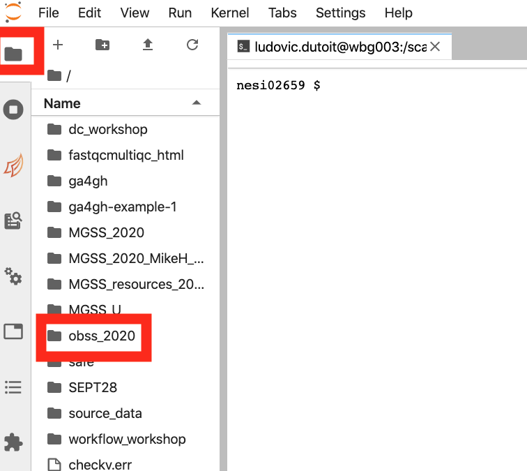
Let’s look at this FastQC report together:

• What is this weird thing in the per base sequence content from base 7 to 12-13?

• You probably noticed that not all of the data is high quality (especially if you check the ‘Per base sequence quality’ tab!). In general with next generation sequencing, you want to remove the lowest quality sequences from your data set before you proceed. However, the stringency of the filtering will depend on the final application. In general, higher stringency is needed for de novo assemblies as compared to alignments to a reference genome. However, low quality data can affect downstream analysis for both de novo and reference-based approaches, producing false positives, such as errant SNP predictions.
We will use the Stacks’s program process_radtags to remove low quality sequences (also known as cleaning data) and to demultiplex our samples. Here is the Stacks manual as well as the specific manual page for process_radtags on the Stacks website to find information and examples.

• Get back into your dataprep folder by running cd ../ in the terminal (hint: if you are lost use pwd to check where you are).

• It is time to load the Stacks module to be able to access the process_radtags command. Find the module and load it (hint: Do for Stacks what we did above for FastQC).

• You will need to specify the set of barcodes used in the construction of the RAD library. Remember, each P1 adaptor in RAD has a particular DNA sequence (an inline barcode) that gets sequenced first, allowing data to be associated with individual samples.

• To save you some time, the barcode file is at: /nesi/project/nesi02659/obss_2020/resources/day3/lane1_barcodes.txt Copy it to the dataprep where you currently are.

• Have a look at the inside of this file using the less command. Normally, these sample names would correspond to the individuals used in a particular experiment (e.g. individual ID etc), but for this exercise, samples are named in a simple way.

• Based on the barcode file, can you check how many samples were multiplexed together in this RAD library? (hint: you can count the lines in the file using wc -l lane1_barcodes.txt)

• Have a look at the help online to prepare your process_radtags command. You will need to specify:
- the restriction enzyme used to construct the library (SbfI)
- the directory of input files (the lane1 directory)
- the list of barcodes (lane1_barcodes.txt), the output directory (samples)
- the fact that the input files are gzipped
- finally, specify that process_radtags needs clean, discard, and rescue reads as options of process_radtags
• You should now be able to run the process_radtags command from the dataprep directory using these options. It will take a couple of minutes to run. Take a breath or think about what commands we’ve run through so far.

• The process_radtags program will write a log file into the output directory. Have a look in there. Examine the log and answer the following questions:
- How many reads were retained?
- Of those discarded, what were the reasons?
- In the process_radtags log file, what can the list of “sequences not recorded” tell you about the barcodes analysed and about the sequencing quality in general?

Well done! Take a breath, sit back or help your neighbour, we will be back shortly!

Back to homepage