De-novo assembly without a reference genome
Developed by: Julian Catchen, Nicolas Rochette
Adapted by: Ludovic Dutoit
Goals
- Learn to call SNPs without a reference genome and to optimise the procedure
- Learn to run SLURM scripts
Introduction
In this second exercise we will be working on threespine stickleback data sampled from throughout Oregon, on the West Coast of the United States. These sticklebacks can be found in a number of habitats from costal marine and freshwater habitats, to inland river habitats, to high mountain lakes in the interior of Oregon. We want to understand how these populations relate to one another and in this exercise, you will examine three of these populations: a coastal marine population, a coastal freshwater, and an inland river population. Our data consist of 30 samples in these three populations. For more information on the background of this study, see Catchen et al, 2013.
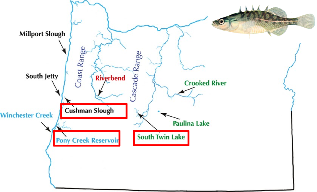
Map of Stickleback populations
Without access to a reference genome, we want to assemble the RAD loci and examine population structure. However, before we can do that, we want to explore the de novo parameter space in order to be confident that we are assembling our data in an optimal way. Stack (i.e. locus) formation is controlled by three main parameters:
-m : the minimum amount of reads to create a locus (default: 3)
-M : the number of mismatches allowed between alleles of the same locus (i.e. The one we want to optimise)
-n : The number of mismatches between between loci between individuals (default 1)
If that does not make sense or you would like to know more, have a quick read of this explanation from the manual.
Here, we will optimize the parameter M (description in bold above) using the collaborative power of all of us here today! We will be using the guidelines of parameter optimization outlined in Paris et al. (2017) to assess what value for the M parameter recovers the highest number of polymorphic loci. Paris et al. (2017) provides a description of this approach:
“After putative alleles are formed, stacks performs a search to match alleles together into putative loci. This search is governed by the M parameter, which controls for the maximum number of mismatches allowed between putative alleles […] Correctly setting M requires a balance – set it too low and alleles from the same locus will not collapse, set it too high and paralogous or repetitive loci will incorrectly merge together.”
As a giant research team, we will run the denovo pipeline with different parameters. The results from the different parameters will be shared using this Google sheet. We’ll be able to use the best dataset downstream for population genetics analyses and to compare with a pipeline that utilises a reference genome.
Build your denovo_map.pl command
-
In your
GBSworkspace, create a directory calledoutput_denovoto contain the assembled data for this exercise. -
To avoid duplicating the raw data for each of us, we will use a link to the source data. This effectively creates a shortcut to another path without copying all the files.
ln -s /path/you/want/to/linkwill create a shortcut to a given path right where you are! The raw data is in/scale_wlg_persistent/filesets/project/nesi02659/obss_2020/resources/day3/oregon_stickleback/Using the above explanation, create a link to this folder right here! -
Run Stacks’ denovo_map.pl pipeline program according to the following set of instructions. Following these instructions you will bit by bit create the complete
denovo_map.plcommand:• Make sure you load the
Stacksmodule (you can check if you have already loaded it usingmodule list)• Get back into the
GBSfolder if you wandered away.• Information on denovo_map.pl and its parameters can be found online. You will use this information below to build your command.
• We want Stacks to understand which individuals in our study belong to which population. Stacks uses a so-called population map. The file contains sample names as well as populations. The file should be formatted in 2 columns like this. All 30 samples are at the file path below. Copy it into the
GBSfolder you should currently be in. Note that all the samples have been assigned to a single “dummy” population, ‘SINGLE_POP’, just while we are establishing the optimal value of M in this current exerise./nesi/project/nesi02659/obss_2020/resources/day3/popmap.txt• Make sure you specify this population map to the denovo_map.pl command.
• Specify
-r/--min-samples-per-popat 0.8, requiring 80% of samples to have a given locus for it to be kept in the output.• In groups of 2, it is time to run an optimisation. So have a sip until your neighbor catch up or help them along. There are three important parameters that must be specified to denovo_map.pl, the minimum stack/locus depth (
m), the distance allowed between stacks/loci (M), and the distance allowed between catalog loci (n). Choose which values ofMyou want to run (M<10), not overlapping with parameters other people have already chosen, and insert them into this google sheet.You can vary M (between 1 and 8). If you find most M values already running in the spreadsheet, you could vary -r away from 0.8 to see how that affect the results.• Set
n= toM, so if you setMat 3, setnat 3.• Set
mat 3, it ios the default parameter, we are us being explicit here for anyone (including ourselves), reading our code later.• You must set the
output_denovodirectory as the output, and use 4 threads (4 CPUs: so your analysis finishes faster than 1!).• Specify the path to the directory containing your sample files (hint use your
oregon_stickleback/link here!). The denovo_map.pl program will read the sample names out of the population map, and look for them in the samples directory you specify.• Your command should be ready, try to execute denovo_map.pl (part of the Stacks pipeline).
• Is it starting alright? Good, now Use
control + cto stop your command -
Running the commands directly on the screen is not common practice. You now are on a small server which is a reserved amount of resources for this workshop and this allows us to run our commands directly. On a day to day basis, you would be logging in on the login node of NeSI’s Mahuika (i.e. the place you reach when you login) and running jobs using a batch script. The batch script (or submission script) accesses all the computing resources that are tucked away from the Mahuika login node. This allows your commands to be run as jobs that are sent out to computing resources elsewhere on Mahuika, rather than having to run jobs on the login node itself (which can slow down people logging in/transferring files if the login node is busy running peoples’ jobs!). We will use this denovo_map.pl command as a perfect example to run our first job using a batch script.
• copy the example jobfile into this directory. The example is at:
/nesi/project/nesi02659/obss_2020/resources/day3/denovojob.sh• Open it with a text editor, have a look at what is there. The first line is
#!/bin/bash -e: this is a shebang line that tells the computing environment that language our script is written in. Following this, there are a bunch of lines that start with#SBATCH, which inform the system about who you are, which type of resources you need, and for how long.• For a few of the
#SBATCHlines, there are some spaces labelled up like<...>for you to fill in. These spaces are followed by a comment starting with a#that lets you know what you should be putting in there. With this information, fill in your job script.• Once you are done, save it. Then run it using:
sbatch denovojob.sh• You can check what the status of your job is using:
squeue -u <yourusername>• We used a few basic options of sbatch, including time, memory, job names and output log file. In reality, there are many, many, more options. Have a quick look at
sbatch --helpout of interest. NeSI also has its own handy guide on how to submit a job here.• Once your job is no longer listed in
squeueis empty, it has finished and what would have printed to your screen has instead printed into denovo.log. Your job should take about 1 hour to run, so in the meantime, sit back and relax, we’ll get back to this after lunch!
Analysing the data from our collaborative optimisation
Examine the Stacks log and output files when execution is complete. You should find all of this info in output_denovo/denovo_map.log
• After processing all the individual samples through ustacks and before creating the catalog with cstacks, denovo_map.pl will print a table containing the depth of coverage of each sample. Find this table in output_denovo/denovo_map.log: what were the depths of coverage?
• Examine the output of the populations program in the file populations.log inside your output_denovo folder (hint: use the less command).
• How many loci were identified?
• How many variant sites were identified?
Enter that information in the collaborative Google Sheet
• How many loci were filtered?
• Familiarize yourself with the population genetics statistics produced by the populations component of stacks populations.sumstats_summary.tsv inside the output_denovo folder
• What is the mean value of nucleotide diversity (π) and FIS across all the individuals? [hint: The less -S command may help you view these files easily by avoiding the wrapping]
Congratulations, you obtained variants :)